Parameter Tuning Guide

Introduction to TitanQ Tuning

TitanQ does much of the heavy lifting to solve your very challenging problems. To allow the greatest flexibility, however, some knobs have been exposed to allow the best performance across a variety of problems. This guide intends to explain these knobs, and give insight into how best to tune TitanQ to deliver the best results for the specific problem at hand.

Each parameter in this guide is labeled with one or both of the following indicators:

Quantum-Inspired

indicates that the parameter is used in the quantum-inspired optimization approach.

LP/QP

indicates that the parameter applies to quadratic and linear programming solver.

If a parameter has both indicators, it is utilized by both solvers. For more information about the solver classes, refer to our solvers description

Required parameters

timeout_in_secs

Quantum-Inspired

LP/QP

The timeout for the solve request is problem size dependent. Generally large problems should have larger timeouts. If your problems are < 1000 variables something like a 30 second timeout is reasonable. If your problems are > 10000 variables, a 60 second minimum timeout is recommended.

variable_types

note

LP/QP

  solver only supports continuous variables. However, if there is a mix of continuous an other variable types  

Quantum-Inspired

  solver will be used instead.

List of chars specifying the variable type for each respective problem variable.

• 'b' - binary.
  Quantum-Inspired
• 'i' - integer.
  Quantum-Inspired
• 'c' - continuous.
  Quantum-Inspired
  LP/QP

Model Hyperparameters

Model hyperparameters are mathematical adjustments that help the system’s stochastic sampler converge to optimal solutions. TitanQ’s two hyperparameters, beta & coupling_mult, drastically affect the resulting solution identified and therefore should be the 1st place to investigate when tuning.

beta

Quantum-Inspired

To best explore the state space for optimal solutions, a scaling factor for the problem can be used. An array of scaling factors, here as beta, helps ensure that local minima are able to be escaped from as well as respect for problem constraints if present.

To find the endpoints and values of this array of beta, we usually look at the inverse of beta (we refer to this as temperature) as this directly maps to the values in the weights and bias matrices.

For unconstrained problems:

• Tmin = min(abs(weights[weights != 0]), abs(bias[bias != 0]))
• Tmax = median(abs(weights[weights != 0]), abs(bias[bias != 0]))

For constrained problems:

• Tmin = min(abs(weights[weights != 0]), abs(bias[bias != 0]))

• Tmax = 10*max_row_sum

  In this case, “max_row_sum” refers to the maximum sum of values in a particular row of your weights matrix/bias vector. Generally this will yield a much higher Tmax than the unconstrained problems.

From these endpoints, interpolation can be used to fill the array with appropriately spaced values as shown below

• beta = 1.0 / np.geomspace(T_min, T_max, num_chains)

Some notes & observations on setting the Tmin and Tmax values when generating the beta vector are as follows:

• Tmin
  • If given a set of hyperparameters, decreasing Tmin to a very small number such as 0.0005 usually doesn’t damage the solution quality (sometimes improves it slightly).
• Tmax
  • Sometimes, Tmax has an upper fall off value. I.e. setting Tmax beyond a certain value gives degenerate solutions.
  • Sometimes, increasing Tmax beyond a certain peak value no longer improves solutions.
    • These high temperature chains are essentially useless since they all trickle down to the lower temp ones.

While defining individual values for the beta array is possible, it is not recommended as proper spacing between values is important, and is well handled by either linear spacing (np.linspace with Numpy) or geometric spacing (np.geomspace with Numpy) depending on the problem.

coupling_mult

Quantum-Inspired

To map problems onto the TitanQ system, we use a mapping between the initial problem graph, and the graph that is actually solved on the hardware (a bipartite RBM graph). This is the mapping from A) to B) in the figure below.

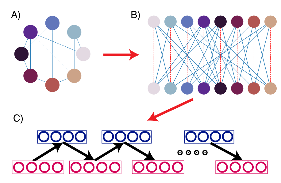
This is enforced as a soft constraint between the logical nodes and the physical nodes, where there are 2 physical nodes for each logical node (For more context, see this example of the difference between logical and physical nodes https://link.springer.cocm/article/10.1007/s11128-008-0082-9 ). This constraint is represented by the red dotted line in the above figure B). The coupling_mult parameter sets the strength of this constraint and is usually set to a value between [0, 1]. In most cases we have found that setting it to coupling_mult=0.3 gives a sufficiently good solution quality and is a good starting point.

When the coupling_mult is too low, the solution to the problem diverges from the solution returned by the hardware system. This is because the constraint is not strong enough in the problem, and the solution is solving the “wrong” problem. When coupling_mult is too high, the system is solving the correct problem, but may do so very slowly, and converge slowly. This is OK in many cases, as you will receive an answer that is “good enough”. We suggest starting with a coupling_mult value that is slightly too high and working downwards.

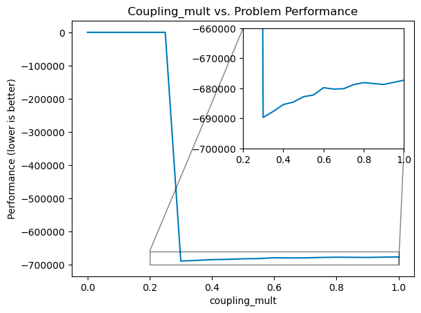
As a strategy for setting this parameter, we have usually started at the value of coupling_mult=0.3, and adjusted from there. If the solution quality is very bad then usually coupling_mult is too low, and we must raise it. If the solution is reasonable but we suspect a better one exists, then we can test this by reducing coupling_mult gradually until we suddenly start seeing degraded solution performance. The best solutions will be produced when coupling_mult is set just before this “fall-off” point, represented by the graph below. In this graph, you can see that setting coupling too low is catastrophic in solution quality, but setting coupling too high simply means slightly sub-optimal solutions.

For further reading, you can see our paper on RBM-based mappings (https://arxiv.org/pdf/2008.04436), specifically discussions around the C parameter and graph embeddings.

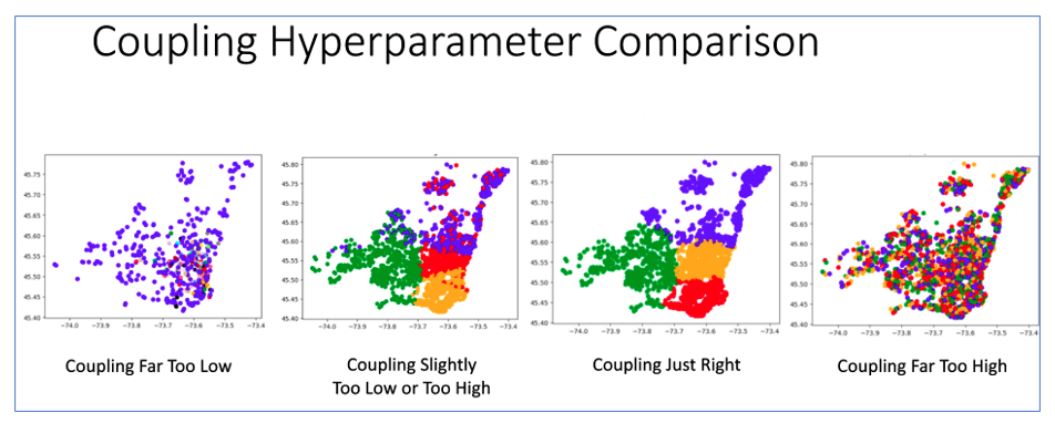
A visual example of coupling_mult set too low or too high is included below as seen in our support for Clustering:

In summary,

• Most optimal coupling_mult values are between 0.03 and 0.5, and the maximum coupling seen for most problems is ~1.
  • We recommend starting with coupling_mult=0.3.
• Solutions tend to improve as coupling_mult decreases, up until a “fall-off” point.
• As coupling_mult gets closer and closer to the fall-off value from above, solutions tend to improve.
• When coupling_mult gets too close to the fall-off value, an increasing fraction of runs begin to give degenerate solutions.
  • These degenerate solutions have very high energies (which is bad in the context of minimization) compared to other runs.
  • These solutions tend to be all zeros or all ones.
• A common tuning strategy is to iteratively lower coupling_mult as much as possible before solutions become degenerate.

penalty_scaling

Quantum-Inspired

note

If null, a value will be inferred from the objective function of the problem.

Scaling factor for constraint penalty violations. Increasing this value results in stronger constraint enforcement at the cost of increasing the odds of becoming trapped in local minima.

precision

Quantum-Inspired

Some problems may need a higher precision implementation to converge properly such as when problem weights exhibit a high dynamic range. This flag allows this higher precision (but slightly slower speed) implementation to be used when "high" is set. Setting "standard" uses a medium precision perfect for general use and offering the best speed/efficiency. The default setting "auto" will inspect the problem passed in and determine which of "high" or "standard" precision to use based on internal metrics.

optimality_gap

LP/QP

The optimality_gap parameter defines the required level of accuracy for the solver to consider a solution acceptable. It specifies how close the solver must get to the best possible (and likely optimal) solution before terminating.

The solver evaluates two main conditions to determine whether the solution meets the required accuracy:

1. Scaled Error: The solver computes an error metric that quantifies the distance from the optimal solution. If this error is smaller than the specified value, the solver considers the solution sufficiently accurate.
2. Additional Criteria: The solver also checks two other conditions.
3. Dual Feasibility: This measures how well the solution satisfies the dual feasibility conditions.
4. Constraint Violation: This measures the degree to which the solution violates the problem's constraints.

If all these conditions are met, the solver terminates successfully. The optimality_gap parameter should be a small positive number (greater than zero). The exact termination condition varies across solvers. The default value is 1e-4 for the LP/QP solver, but it can be adjusted based on the specific requirements of the problem.

note

The LP/QP solver is designed to explore the solution space defined by the provided model until it finds a solution that is close than the specified gap, as it's not always feasible to terminate with the exact gap requirement.

System Parameters

System parameters are directly related to solve request efficiency and resource utilization. These are not mathematically related to the problem to be solved, and instead define the configuration of the solve request to be launched.

num_buckets

Quantum-Inspired

note

num_buckets parameter is only used when there are continuous variables in the problem.

The buckets strategy consists in dividing the range of values of a continuous variable into the specified number of buckets. Each bucket is of equal size (for instance, if your variable can take values between -1000.0 and +1000.0, and the specified number of buckets is 10, each bucket will be of size 200.0). The algorithm will explore the solution space by moving from one bucket to an adjacent one, finding the best solution in the bucket each time. For the strategy to work properly, there must be at most one optimum (either a maximum or a minimum) in each bucket.

In general, the more complex the problem, the greater the number of buckets is needed to find quality solutions. More difficult problems (highly non-convex and heavily constrained) will generally require more buckets to escape local minima.

Below are some recommendations:

• For easy problems, start with 1 bucket and increment up to 10 buckets to see if there is an improvement on the solution quality. If it seems to help, keep increasing the number of buckets by 10 at a time until 100. Then 100 at a time until 1000.
• Keep in mind that the number of samples taken when using buckets is greatly diminished because each sample implies a search within a bucket which takes some computing time. The quality of the solution obtained should, however, be significantly improved.

num_chains & num_engines

Quantum-Inspired

LP/QP

The number of chains and engines determine how many copies of the problem to launch simultaneously. The num_chains is the same as the length of beta as each chain will be assigned one value from the beta array. The num_engines is the number of independent batches of chains to run in parallel. The number of engines will be the same as the number of solutions returned, as the best chain from each engine will be returned.

Smaller total number of chains (num_chains * num_engines) will result in more samples taken for the same timeout. This means that the absolute potential best solution quality could be higher. However, running more chains in parallel will guarantee a higher average solution quality, as while fewer samples are taken in each chain, there are more chains exploring the space.

Below are some recommendations:

• num_chains = 16, is usually the minimum, but higher granularity may be needed.
• num_chains = 32, is usually a good value for this parameter. Larger than this usually does not have much benefit, though up to 64 has been seen to be effective.
• Hyperparameters may need to be retuned with a new num_chains value.
• A previous misconception was that it would be better to have more than 32 chains if the gap between Tmin and Tmax was very large, e.g. Tmin = 2 and Tmax = 32000. Increasing num_chains did not help for most cases.
• num_chains * num_engines = 256 for best results. For num_chains=32, num_engines=8. The system will return 8 solutions back to you, and you can decide which solution is best by your own metrics (constraint violations, minimal error, etc.).

Other Parameters

constant_term

Quantum-Inspired

LP/QP

This parameter represents a fixed value added to the final computed objective value.

Example: Suppose the objective function to minimize is 'f(x) = x^2 + 2x + 4' and 'x' is a binary variable.

The optimal solution would be 'x = 0' resulting in an optimal objective function value of 'f(x) = 4'. However, the solver ignores constant terms and only seeks to minimize 'f(x) = x^2 + 2x'. This would typically yield f(x)=0 by default with the optimal solution of 'x = 0'. constant_term should be set to 4 to yield an objective function value of 'f(x) = 4'.

Potential Tuning Strategies

Sandwich Tuning

1. Begin with a decent set of hyperparameters (as suggested above).
2. Begin with num_chains=16 and num_engines=8.
3. Decrease Tmin to a very low number such as 0.0005.
4. Increase Tmax to a higher number (100-200 frequently seen).
5. Iteratively lower coupling_mult right before solutions become degenerate (find the “fall-off” point).
6. Take turns increasing Tmin and decreasing Tmax until solution stops improving.
   1. If solutions start to become degenerate, consider readjusting coupling_mult, usually by raising it in steps of 0.01 magnitude.
7. Increase num_chains to a maximum of approximately 64 to see if better temperature resolution improves quality.
   1. If so, repeat steps 1-6 with new system configuration.

This strategy makes the following assumptions:

• Tmin below a certain value stops improving solution quality.
• Tmax above a certain value stops improving solution quality.
• The fall-off point for coupling_mult is not dependent (or low dependence) on Tmin or Tmax.

3rd Party Packages (Optuna)

1. Run Optuna with a 1 min timeout and 100 trials (300 or more trials is even better).
2. Take either the best performing set of hyperparameters (min), or the “mean of the sets of hyperparameters that gave the most consistently good solutions”.
3. Run these hyperparameters on TitanQ with the same 1 min or longer timeout.
4. Using Optuna with shorter timeout and more trials almost always performed better than longer timeout and fewer trials.